Inventory Optimization

Optimization

Every company has the challenge of matching its supply volume to customer demand. How well the company manages this challenge has a major impact on its profitability. Inventory optimisation is a method of balancing capital investment constraints and service-level goals over a large assortment of stock-keeping units (SKUs), while taking demand and supply volatility into account.

ABC Analysis

Inventory optimization in a supply chain, ABC analysis, is an inventory categorization method, which consists of dividing items into three categories, viz., A, B and C. A is the most valuable item, while C is the least valuable one. This method aims to draw managers’ attention to the critical few (A-items) and not the trivial many (C-items).

Inventory optimization is critical to keeping costs under control within the supply chain. Yet, to get the most from management efforts, it is efficient to focus on items that cost the most to the business.

The Pareto principle states that 80% of the overall consumption value is based on only 20% of total items. In other words, demand is not evenly distributed between items; top sellers vastly outperform the rest.

The ABC approach states that, when reviewing inventory, a company should rate items from A to C, basing its ratings on the following rules:

A-items goods’ annual consumption value is the highest. 70-80% of the annual consumption value of the company typically accounts for only 10-20% of total inventory items.

C-items are, on the contrary, items with the lowest consumption value. 5% of the annual consumption value typically accounts for 50% of total inventory items.

B-items are intermediate items, with a medium consumption value. 15-25% of annual consumption value typically accounts for 30% of total inventory items.

The annual consumption value is calculated with the formula: (annual demand) x (item cost per unit).

Through this categorization, the supply manager can identify inventory hotspots, and separate them from the rest of the items, especially those that are numerous but not that profitable.

Commerce Example

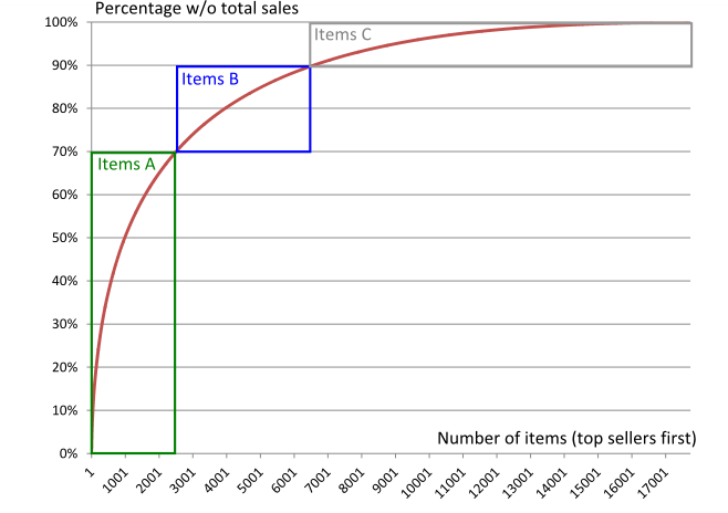
The graph above illustrates the annual sales distribution of USA eCommerce in 2011 for all products that have been sold at least once. Products are ranked by starting with the highest sales volumes.

Out of 17 000 references:

• The top 2 500 products (Top 15%) represent 70% of the sales.
• The next 4 000 products (Next 25%) represent 20% of the sales.
• The bottom 10 500 products (Bottom 60%) represent 10% of the sales.

Click here to view a video on the 8 best practices for inventory management.

Economic Order Quantity

Economic Order Quantity (EOQ) is the order quantity of inventory that minimizes the total cost of inventory management.

The two most important categories of inventory costs are ordering costs and carrying costs. Ordering costs are costs that are incurred when obtaining more inventories. They include costs incurred on communicating the order, transportation costs, etc. Carrying costs are the costs incurred on holding inventory in hand. They include the opportunity cost of money held in inventories, storage costs, spoilage costs, etc.

Ordering costs and carrying costs are quite different to each other. If we need to minimize carrying costs, we must place small orders, which increases the ordering costs. If we want to minimize our ordering costs, we must place fewer orders in a year, and this requires placing larger orders which, in turn, increases the total carrying costs for the period.

We need to minimize the total inventory costs, and the EOQ model helps us just do that.

Total inventory costs = Ordering costs + Holding costs

By taking the first derivative of the function, we find the following equation for minimum cost:

EOQ = Square root (SQRT) (2 × Quantity × Cost Per Order / Carrying Cost Per Unit)

Example:

ABC Ltd. is engaged in the sale of footballs. Its cost per order is R 400 and its carrying cost unit is R 10 per unit per annum. The company has a demand for 20 000 units per year. Calculate the order size, the total orders required during a year, the total carrying cost, and the total ordering cost for the year.

Solution:

EOQ = SQRT (2 × 20 000 × 400/10) = 1,265 units

The annual demand is 20,000 units so the company will have to place 16 orders (= annual demand of 20,000 divided by order size of 1,265). The total ordering cost is R 6 400 (R 400 multiplied by 16).

The average inventory held is 632.5 ((0+1,265)/2) which is the total carrying cost of R 6 325 (i.e. 632.5 × R 10).