Descriptive Measures

Presentation methods are in themselves not sufficient for business decision-making. Having gained an impression of the overall characteristics of a data set, we must now examine the data in greater detail to develop a more precise, quantitative description of the data. Numbers used to describe the data sets are called descriptive measures. Statistics are summary measures used to describe a sample, and populations are described by parameters.

The most important measures of description will now be discussed:

Measures of Central Tendency

Click here to view a video that explains what Central Tendency is.

These measures are numbers that represent the typical or middle values in a distribution. In most cases, the data tend to cluster in the middle around some value that is often referred to as an average. There are many types of averages, each with its own characteristics. The most commonly used averages are the arithmetic mean, the median and the mode.

Click here to view a video that explains Mode, Median, Mean, Range, and Standard Deviation.

Click here to view a video that explains the Mean, Median, and Mode of Grouped Data and Frequency Distribution Tables Statistics.

The Arithmetic Mean

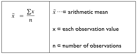
This is the most commonly used measure of central tendency and is often being referred to as the average or the mean. It is the sum of the values of a data set divided by the number of observations.

Calculation of a mean:

The Median

The median is the value that occupies the middle position of a group of numbers arranged in numerical order. It divides the bottom 50% of data from the top 50%.

Calculation of the median:

Median position = n + 1 / 2

Example:

Number list: 4 5 10 12 50 60 80

Position of the median: n + 1 / 2 = 7 + 1 / 2 = value 4

Median = 12

Note: for a shortlist the median can simply be read off the list, but for a long number list, you will need to use the formula.

The Mode

The mode is the number that occurs the most often in a data set; it is the number with the highest frequency.

For ungrouped data, the model requires no calculation and can easily be obtained from a number list. If there is no number that occurs more frequently than the others, there is no mode, but this is not the same as a mode of 0. A set of data may also have more than one mode and is then said to be bi-modal or multi-modal.

Example:

The commission earnings of your salespeople were as follows for the previous month:

R5 000    R5 200   R5 200   R5 700   R8 600

The modal commission was R5 200

Which Measure of Central Tendency to Use When?

Mean:  Commonly used and easy to calculate.

Every numerical set has a mean.

It is unique – every data set has only one mean.

Reliable – because it reflects all the values of the data set.

Median: It is a better measure of central tendency when data is much skewed, i.e. extreme values do not affect the median as strongly as the mean.

Easy to read off a set of data.

Mode: Not often used in statistics.

Measures of Dispersion

Two data sets can have the same mean, and yet be very different if one is more spread out than the other. To describe this difference quantitatively, we use a measure of dispersion, which indicates the amount of variation in a data set. Some commonly used measures of dispersion are the range, the standard deviation and the variance.

The Range: The range is the difference between the highest and the lowest values in a data set. It measures the distance across the entire set of data:

Range = maximum value - minimum value

The Standard Deviation: The standard deviation is the most widely used measure of dispersion, and measures differences from the mean. To prevent negative deviations from the mean, cancelling positive deviations, the deviations are squared. The standard deviation is useful in statistics because:

• Most distributions in statistics are described by their mean and standard deviation.
• The measuring unit is the same as the mean (Rands, minutes, metres, etc.).
• The larger the standard deviation, the larger the variation of data. A standard deviation of zero means there is no variation.

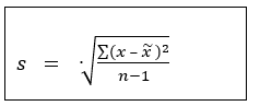
The calculation of the standard deviation:

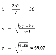
Example:

The errors on seven invoices were recorded as follows:

The Variance(s²)

The variance is the standard deviation squared (s²). Although this is a very popular description of data, the main drawback is that the unit of measurement is also squared. If the standard deviation is equal to 5.25 hours, the variance will be 27.56 hours squared.

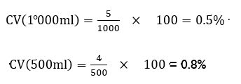
The Coefficient of Variation (CV)

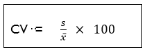
The coefficient of variation is the ratio, expressed as a percentage of the standard deviation to the mean. In practice, the CV can be used to compare two or more sets of data with different means, sample sizes of measurement units.

The formula for CV:

Example:

A manufacturing company produces a product in two sizes: a 1 000ml bottle and a 500ml bottle. Because of mechanical variability in the filling machinery, there is a standard deviation of 5ml and 4 ml respectively. The more consistent machine is the one with the lower CV.

Measures of Shape

The shape and distribution can be described by:

• Its symmetry or lack of it (skewness);
• Its peakedness (kurtosis).

Skewness (SK)

The skewness of a set of data relates to the histogram or polygon that could be drawn from the data. Although it is possible to create arithmetic measures of skewness we will not go into such detail for the purpose of this program.

Skewness describes the relationship between the locations of the mean, median and mode and the shape of the distribution. Such values are known as extreme values or outliers. The mode is not influenced by extreme values at all and stays at the peak of the distribution. The median being dependant on the number of values in the data set rather than on the size of those values is less sensitive than the mean and ends up somewhere between the mode and the mean. The mean is influenced the most by extreme values because the values are included in its computation.

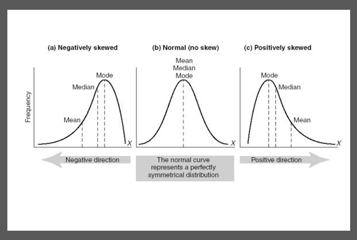
The three forms of skewness can be interpreted as follows:

Normal/symmetrical distributions: The left half is a mirror image of the right half. The mode, median and mean will be on the same line in the middle. There are no extreme values to pull the mean away from the bulk data.

Positive skewness: Occurs when the mean exceeds the median and both the mean and median are greater than the single-mode. The mean exceeds the median because a few large values in the upper tail pull the mean up.

Negative skewness: Occurs when the mean is less than the median, and the single-mode exceeds both the mean and the median. The mean is less than the median because a few low values in the lower tail pull the mean down.

Click here to view a video that explains what skewness is.